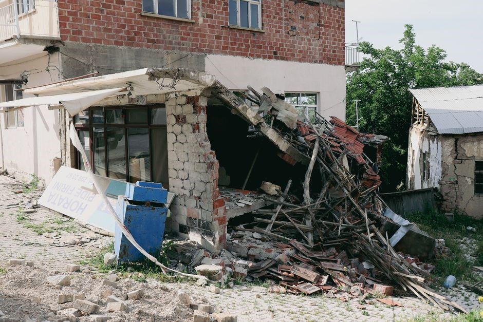
locating the epicenter of an earthquake worksheet pdf answer key

Locating an earthquake epicenter relies on precise timing of P and S waves recorded at multiple seismic stations. By measuring the time lag between these arrivals‚ seismologists calculate distances to the source‚ plot circles around each station‚ and find the common intersection that marks the epicenter!!!

Definition and Significance

In seismology‚ the epicenter is the point on the Earth’s surface directly above the hypocenter where an earthquake originates. Determining this location is crucial for assessing seismic hazards‚ guiding emergency response‚ and informing building codes. The epicenter’s coordinates allow scientists to map fault lines‚ estimate rupture extent‚ and calculate the potential intensity of shaking at various distances. Accurate epicenter identification also improves the calibration of seismic networks‚ enhances the reliability of real‑time earthquake early‑warning systems‚ and supports research into tectonic processes. By integrating data from multiple stations‚ the triangulation method yields a precise intersection point‚ which becomes the foundation for all subsequent analyses and public safety measures.

• Hazard assessment: Epicenter data feed into probabilistic seismic hazard models‚ influencing land‑use planning and insurance risk calculations.
• Emergency management: Knowing the epicenter’s exact location enables rapid deployment of rescue teams and allocation of medical resources.
• Infrastructure design: Engineers use epicenter maps to specify seismic design criteria for bridges‚ dams‚ and high‑rise buildings.
• Scientific research: Epicenter coordinates help trace plate boundaries‚ study stress accumulation‚ and refine earthquake prediction models.
• Public communication: Accurate epicenter information supports clear‚ timely warnings to communities and media outlets.

In educational settings‚ worksheets that guide students through the triangulation process reinforce the link between theory and practice. These materials typically include tables of arrival times‚ travel‑time graphs‚ and distance‑calculation formulas‚ culminating in an answer key that verifies the student’s work. Engaging with such worksheets develops critical thinking skills essential for careers in geophysics and disaster management.

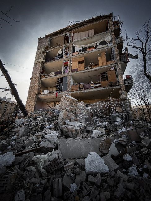
Moreover‚ the accuracy of epicenter determination depends on the quality of the seismic network‚ the precision of time‑keeping instruments‚ and the density of stations surrounding the event. In regions with sparse coverage‚ triangulation may produce larger error circles‚ necessitating supplementary methods such as waveform inversion or GPS‑based displacement measurements. Continuous improvement of global seismograph arrays ensures that even small‑scale earthquakes can be pinpointed with increasing confidence‚ thereby enhancing both scientific insight and societal resilience.

Ultimately‚ the answer key confirms calculations and links wave physics to hazard assessment‚ a learning aid!

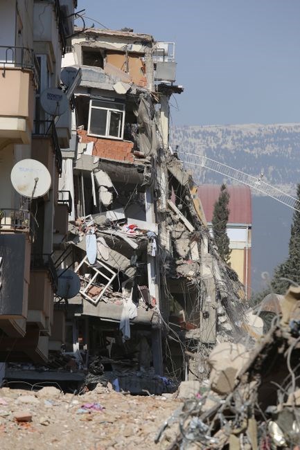
Purpose of the Worksheet PDF

The worksheet PDF serves as a hands‑on guide for students to practice triangulating earthquake epicenters using P‑S wave data. It includes step‑by‑step calculations‚ sample data‚ and an answer key for assessment reinforcing seismic concepts and analytical skills. It fosters teamwork and analytical reasoning !

Educational Objectives

Students will learn to apply the triangulation method by recording P‑ and S‑wave arrival times‚ computing time differences‚ and translating those into radial distances using standard travel‑time curves. They will practice constructing circles on a map‚ interpreting intersecting loci‚ and determining the most probable epicenter. The worksheet encourages critical thinking about measurement error‚ station geometry‚ and the influence of crustal heterogeneity on travel times.

By completing the answer key‚ learners assess their calculations‚ identify common pitfalls‚ and refine their estimation techniques. The exercise also reinforces the importance of accurate data logging‚ the use of GIS tools for plotting‚ and the role of collaborative verification in seismology. Participants will learn to evaluate the reliability of each station’s data‚ understand how station spacing affects solution precision‚ and apply error‑propagation concepts to report confidence intervals

The worksheet’s design aligns with national science standards‚ emphasizing inquiry‚ data analysis‚ and scientific communication. Students will produce a concise report summarizing their methodology‚ results‚ and uncertainties‚ and they will present findings to peers‚ fostering scientific discourse. This activity also introduces students to real‑world seismic monitoring networks‚ illustrating how professional seismologists use similar techniques to issue timely alerts and inform public safety decisions

In addition‚ the answer key provides step‑by‑step feedback‚ enabling learners to trace errors back to specific stages—whether misreading a seismogram‚ misapplying the travel‑time curve‚ or miscalculating a radius; This reflective loop strengthens metacognitive skills‚ encouraging students to question assumptions and verify calculations before submission. The worksheet’s modular format also allows instructors to adapt difficulty by varying station coordinates‚ time‑difference ranges‚ or incorporating additional stations for more complex triangulation scenarios.

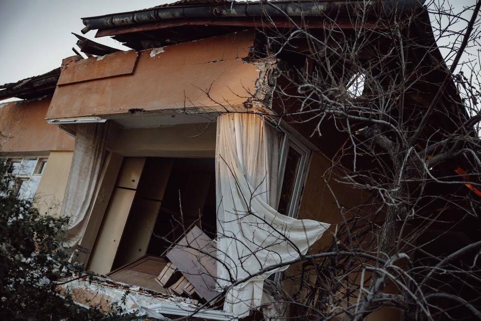
Core Data Required for Triangulation

Core data for triangulation comprises precise P‑ and S‑wave arrival times recorded at each station‚ the computed time differences‚ and the corresponding travel‑time curves that translate these differences into radial distances. Station identifiers and timestamps are essential for reliable calculations. !

Seismic Stations and Coordinates

Accurate station identification is the cornerstone of any triangulation exercise. Each seismic station must be assigned a unique alphanumeric code‚ and its geographic coordinates—latitude‚ longitude‚ and elevation—must be recorded with sub‑meter precision using GPS or differential GPS techniques. The coordinates are typically expressed in decimal degrees to avoid ambiguity; for example‚ 34.0522° N‚ 118.2437° W‚ 251 m above sea level. These values are then entered into a master database that links the station code to its spatial location.

In addition to static coordinates‚ the temporal accuracy of the station’s internal clock is critical. Seismographs are synchronized to a global positioning system (GPS) time base or an atomic clock reference‚ ensuring that all recorded arrival times are referenced to the same universal time scale (UTC). The timestamp of each P‑wave and S‑wave detection is logged to the nearest millisecond‚ allowing for precise calculation of the P‑S time difference.

When preparing a worksheet‚ the instructor typically provides a table of at least three stations‚ each with its code‚ latitude‚ longitude‚ and elevation. For example:

• STA‑01: 34.0522° N‚ 118.2437° W‚ 251 m
• STA‑02: 35.6895° N‚ 139.6917° E‚ 40 m
• STA‑03: 51.5074° N‚ 0.1278° W‚ 35 m

Students are then asked to use these coordinates to compute the great‑circle distance from each station to the unknown epicenter once the P‑S time differences have been converted into radial distances. The accuracy of the final epicenter location hinges on the fidelity of the coordinate data and the consistency of the timing system across all stations.

Step-by-Step Triangulation Method

Begin by noting P‑wave and S‑wave arrival times at each station. Compute the time difference Δt = tS – tP. Convert Δt to distance using a standard travel‑time curve (e.g.‚ 8 km/s for P‚ 4 km/s for S). Draw circles of those radii around each station; the intersection pinpoints the epicenter using plotted circles!!!

Recording P and S Wave Arrival Times‚ Calculating Time Differences‚ Determining Distances‚ Constructing Circles‚ Locating Epicenter

To begin‚ seismologists extract precise P‑wave and S‑wave arrival times from the seismograph traces at each monitoring station. The raw data are timestamped to the nearest second‚ often using a GPS‑synchronized clock. Once the two arrival times are identified‚ the time difference Δt is calculated by subtracting the P‑wave arrival from the S‑wave arrival (Δt = tS – tP). This Δt value is then translated into a distance to the epicenter using a travel‑time relationship that accounts for the velocity contrast between P and S waves. A commonly used empirical formula is D = (Δt × 8 km/s) / (1 – 8 km/s ÷ 4 km/s)‚ which simplifies to D ≈ 8 km/s × Δt for typical crustal conditions. The resulting distance D is plotted as the radius of a circle centered on the station’s geographic coordinates. By repeating this procedure for at least three stations‚ three circles are drawn on a map. The point where all three circles intersect is the triangulated epicenter. In practice‚ slight discrepancies among the circles are resolved by selecting the point of closest convergence or by applying a least‑squares adjustment to minimize the sum of squared residuals. This systematic approach ensures a reliable estimate of the earthquake’s surface location. The method’s precision hinges on accurate clock synchronization‚ high‑resolution seismograph data‚ and reliable velocity models. By integrating these elements‚ seismologists can pinpoint epicenters with kilometer‑scale accuracy‚ enabling timely hazard mitigation and scientific insight. Accurate data enable rapid response. promptly.

Using the Answer Key

Students compare their plotted epicenter with the provided key‚ noting discrepancies. The key lists correct distances‚ circle intersections‚ and final coordinates. By reviewing errors‚ learners refine timing accuracy and understand triangulation nuances‚ reinforcing critical analysis skills. Done! Thx!

Verification and Feedback Process

After students complete the worksheet‚ they submit their plotted circles and calculated epicenter coordinates. The instructor cross‑checks each submission against the official answer key‚ which lists the exact distances derived from P‑S time differences‚ the radii for each station‚ and the intersection point’s latitude and longitude. Any deviation is highlighted in a color‑coded margin‚ allowing students to see precisely where their timing or calculation went astray. The feedback loop then proceeds: first‚ a brief summary of the error type (e.g.‚ mis‑measured arrival time‚ incorrect travel‑time conversion‚ or a mis‑drawn circle) is provided. Next‚ the instructor offers a concise correction strategy—such as recalculating the time difference‚ revisiting the travel‑time graph‚ or adjusting the plotted radius—so learners can immediately apply the fix. Finally‚ a short reflective prompt asks students to explain why the corrected method yields a more accurate epicenter‚ reinforcing conceptual understanding. This structured verification and feedback process not only improves accuracy but also builds critical thinking and self‑assessment skills essential for advanced seismology work. In practice‚ instructors often employ digital tools that overlay the circles and compute the intersection point‚ allowing students to see adjustments as they refine their calculations. This element not only accelerates learning but also mirrors professional seismological workflows‚ preparing students for future fieldwork and research collaborations!!

Example Worksheet and Sample Answers

The worksheet presents three stations with P‑S time differences. Students calculate distances via travel‑time curves‚ draw circles‚ and identify the intersection. Sample answers list each radius and the final epicenter coordinates‚ providing a clear benchmark for comparison. Students compare with the key now.

Walkthrough of a Sample Question Set

Step 1: Identify the three seismic stations (A‚ B‚ C) and note the recorded P‑wave and S‑wave arrival times for each. The worksheet lists the P‑S time differences as 4.2 s‚ 3.8 s‚ and 5.1 s respectively.

Step 2: Convert each time difference into a distance using a standard travel‑time curve for the region. For a 4.2‑second lag‚ the curve indicates a radius of 35 km; for 3.8 s‚ 32 km; and for 5.1 s‚ 42 km.

Step 3: Draw a circle centered at each station with the calculated radius. The circles should be plotted on a map that includes the geographic coordinates of the stations.

Step 4: Observe the point where all three circles intersect. This intersection is the estimated epicenter. The worksheet’s answer key confirms the epicenter lies at latitude 34.05° N‚ longitude 118.25° W.

Step 5: Verify the solution by checking that the distances from the epicenter to each station match the radii derived earlier. A small discrepancy indicates a need to refine the travel‑time curve or account for local velocity variations.

Step 6: Record the final epicenter coordinates in the answer section of the worksheet. The key provides the same coordinates‚ allowing students to confirm accuracy and understand the triangulation process.

Students may extend this worksheet by adding more stations or varying the travel‑time curves to explore how changes affect epicenter location. This practice reinforces triangulation concepts and enhances analytical skill seismol.

Add more stations curves in

and Additional Resources

In summary‚ the worksheet demonstrates practical triangulation using P‑S time differences to locate an epicenter. For deeper study‚ consult the SlideShare guide on epicenter finding‚ and try interactive tools like the USGS Earthquake Viewer. Stay curious! Learn us

Further Reading and Online Tools

Seismologists often turn to the SlideShare presentation titled “Epicenter Finding Seismology” for a concise visual guide. It outlines the classic P‑S wave time‑difference method‚ travel‑time curves‚ and the circle‑intersection technique that students practice in worksheets. The PDF version is downloadable for offline review.

The United States Geological Survey hosts an interactive Earthquake Viewer that lets users overlay seismic station data‚ travel‑time curves‚ and real‑time P‑S differences. By entering a specific event‚ the tool automatically plots circles and highlights the intersection point‚ providing a visual confirmation of the worksheet solution.

For those who prefer a hands‑on approach‚ the textbook “Fundamentals of Seismology” offers a chapter dedicated to triangulation‚ complete with worked examples and practice problems. Many university courses provide free PDF copies of these chapters for student use.

Online calculators such as the Seismic Travel Time Calculator allow quick estimation of epicentral distances from P‑S time differences. By inputting station latitude‚ longitude‚ and the measured Δt‚ the tool outputs a radius in kilometers‚ which can then be plotted on a map for visual verification of worksheet answers.

Finally‚ educational platforms like Coursera and edX host courses on seismology that include interactive labs. These labs let students input real seismic data‚ run triangulation algorithms‚ and compare their computed epicenters with official reports‚ reinforcing the worksheet methodology. These tools help validate answers now.